
Fundamentals of Thermal Resistance
Fundamentals of Thermal Resistance

Today’s guest blog on the fundamentals of thermal resistance is from Dr. James Stevens, Professor Mechanical Engineering at the University of Colorado. Dr. Stevens specializes in numerical and analytical heat transfer analysis covering both steady-state and transient situations with applications to thermal history, thermal response, electronic cooling, temperature profiles, thermal design, and heat flow rate determination.
The Thermal Resistance Analogy
Thermal resistance is a convenient way of analyzing some heat transfer problems using an electrical analogy in order to make complicated systems easier to visualize and analyze. It is based on an analogy with Ohm’s law which is:
In Ohm’s law for electricity, “V” is the voltage which drives a current of magnitude “I”. The amount of current that flows for a given voltage is proportional to the resistance (Relec). For an electrical conductor, the resistance depends on the material properties (copper tends to have a lower resistance than wood, for example) and the physical configuration (thick short wires have less resistance than long thin wires).
For one-dimensional, steady-state heat transfer problems with no internal heat generation, the heat flow is proportional to a temperature difference according to this equation:
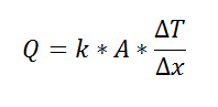
where Q is the heat flow, k is the material property of thermal conductivity, A is the area normal to the flow of heat, Δx is the distance that the heat flows, and ΔT is the temperature difference driving the heat flow.
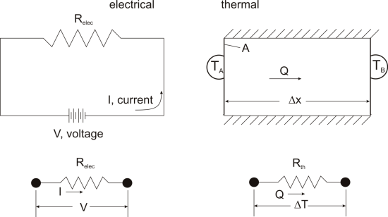
If we create an analogy by saying that electrical current flows like heat, and saying that voltage drives the electrical current like the temperature difference drives the heat flow, we can write the heat flow equation in a form similar to Ohm’s law:  where Rth is the thermal resistance defined as:
 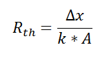 Just as with the electrical resistance, the thermal resistance will be higher for a small cross-sectional area of heat flow (A) or for a long distance (Δx).
Rationale
Now, why bother with all that? The answer is that thermal resistance allows us to solve somewhat complicated problems in relatively simple ways. We’ll talk more about different ways in which it can be used, but first let’s look at a simple case in order to illustrate the benefit.
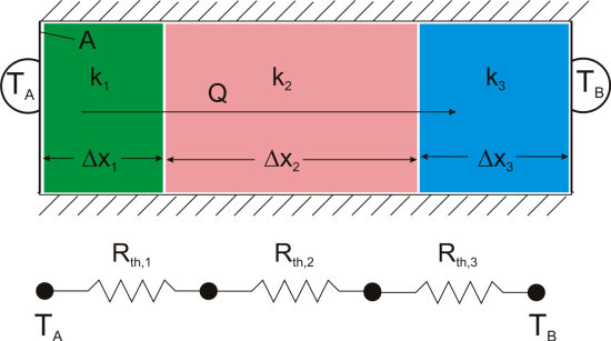
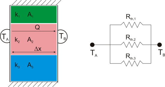
Suppose that we want to calculate the heat flow through a wall composed of three different materials, and we know the surface temperatures at each outside surface, TA, and TB, and the material properties and geometries.
We could write the conduction equation for each material:
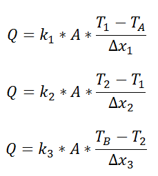
Now, we have three equations, and three unknowns: T1, T2, and Q. For this case it wouldn’t be too much work to algebraically solve for those three unknowns, however, if we use the thermal resistance analogy, we don’t even have to do that much work:
![]()
where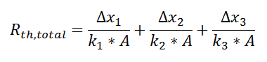
and we can solve for Q in a single step.
Combining Thermal Resistances
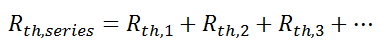
This simple example showed how to combine multiple thermal resistances in series which is the same structure as in the electrical analog:
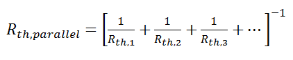
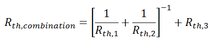
Just like electrical resistances, thermal resistances can also be combined in parallel, or in both series and parallel:
Beyond Conduction
So far, we’ve talked about the thermal resistance associated with conduction through a plane wall. For steady-state, one-dimensional problems, other heat transfer equations can be formulated into a thermal resistance format. For example, examine Newton’s Law of Cooling for convection heat transfer:
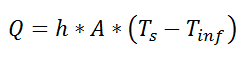
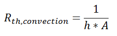
where Q is the heat flow, h is the convective heat transfer coefficient, A is the area over which heat transfer occurs, Ts is the surface temperature on which the convection is taking place, and Tinf is the free-stream temperature of the fluid. As with conduction, there is a temperature difference driving a heat flow. For this case, the thermal resistance would be:
Similarly, for radiative heat transfer from a gray body:
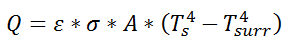
where Q is the heat flow, ε is the emissivity of the surface, σ is the Stefan-Boltzmann constant, Ts is the surface temperature of the emitting surface, and Tsurr is the temperature of the surroundings. By factoring the expression for temperature, the thermal resistance can be written: 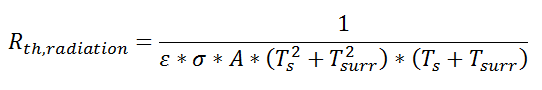
Advantage: Easy Problem Setup
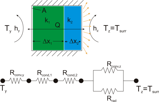
Thermal resistance formulations can make the arrangement of a quite complex problem quite simple to set up. Imagine, for example, that we are trying to calculate the heat flow from a liquid stream of a known temperature through a composite wall to an air stream with convection and radiation occurring on the air side. If the material properties, heat transfer coefficients, and geometry are known, the equation set-up is obvious:
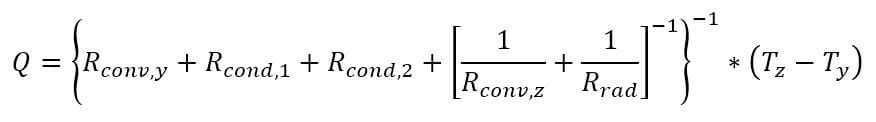
Now, to solve this particular problem might involve an iterative solution since the radiative thermal resistance contains the surface temperature inside of it, but the setup is simple and straightforward.
Advantage: Problem Insight
The thermal resistance formulation has the additional advantage of making it very clear which parts of the model are controlling the heat transfer, and which parts are unimportant, or perhaps even negligible. As a concrete illustration, let’s suppose that in the last example the thermal resistance on the liquid side was 20 K/W, that the first layer in the composite wall was 1 mm thick plastic with a thermal resistance of 40 K/W, that the second layer consisted of 2 mm thick steel with a thermal resistance of 0.5 K/W, and that the thermal resistance for convection to the air was 200 K/W, and the thermal resistance to radiation to the surroundings was 2500 K/W coming from a surface with emissivity of 0.5.
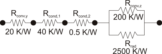
We can understand a lot about the problem by just considering the thermal resistance. For example, since the radiation resistance is in parallel with a much smaller convection resistance, it is going to have a small effect on the overall thermal resistance. Increasing the emissivity of the wall clear to unity would only improve the total thermal resistance by 5%. Or, ignoring radiation completely would cause an error of only 6%. Similarly, the thermal resistance of the steel is in series, and is tiny compared with the other resistances in the system, so no matter what is done to the metal layer it isn’t going to have much effect. Changing from steel to pure copper, for example, would only improve the overall thermal resistance by 0.2%. Finally, it is clear that the controlling thermal resistance is convection on the air side. If it were possible to double the convection coefficient (by, say, increasing the velocity of the air) that step alone would decrease the overall thermal resistance by 36%.
Beyond Plane Wall Conduction
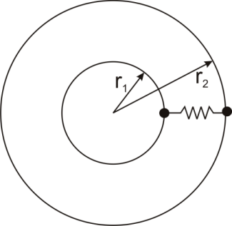
Thermal resistance can also be used for other conduction geometries as long as they can be analyzed as one-dimensional. The thermal resistance to conduction in a cylindrical geometry is:
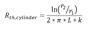
where L is the axial distance along the cylinder, and r1 and r2 are as shown in the figure.
Thermal resistance for a spherical geometry is:
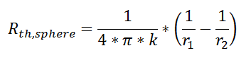
with r1 and r2 as shown in the figure.
Conclusion
Thermal resistance is a powerful and useful tool for analyzing problems that can be approximated as 1-dimensional, steady-state, and that do not have any sources of heat generation.
Please contact Celsia with your next thermal design challenge. We specialize in the design and production of heat sinks using liquid two phase devices: heat pipes and vapor chambers.
Related Links


